What is Faster RCNN?
In this post, I will explain object detection and Faster RCNN which is a machine learning algorithm. We shall start from beginners’ level and go till the state-of-the-art in object detection, understanding the intuition, approach and salient features of each method.
Faster R-CNN was originally published in NIPS. It was presented by Ross Girshick, Shaoqing Ren, Kaiming He and Jian Sun in 2015.
It is one of the famous object detection architectures that uses convolution neural networks like YOLO (You Look Only Once) and SSD ( Single Shot Detector).
Everything started with “Rich feature hierarchies for accurate object detection and semantic segmentation” (R-CNN) in 2014, which used an algorithm called Selective Search to propose possible regions of interest and a standard Convolutional Neural Network (CNN) to classify and adjust them.
It quickly evolved into Fast R-CNN, published in early 2015, where a technique called Region of Interest Pooling allowed for sharing expensive computations and made the model much faster.
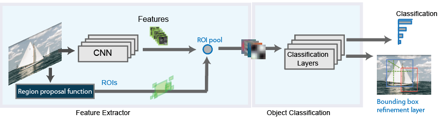
Finally came Faster R-CNN, where the first fully differential model was proposed. Faster R-CNN architecture is complex because it has several moving parts. It all starts with an image, from which we want to obtain:
- a list of bounding boxes.
- a label assigned to each bounding box.
- a probability for each label and bounding box.
The input images are represented as : Height*Depth*Width. Tensors (multidimensional arrays) are passed through a pre-trained CNN. We use this as a feature extractor for the next part.
This technique is very commonly used in the context of Transfer Learning. This technique is mainly used for training a classifier on a small data set using the weights of a network trained on a bigger data set.
We now have a Region Proposal Network (RPN, for short). After CNN computes it results, it is used to find up to a predefined number of regions (bounding boxes), which may contain objects.
The hardest issue with using Deep Learning (DL) for object detection is generating a variable-length list of bounding boxes. When modeling deep neural networks, the last block is usually a fixed sized tensor output.
The variable-length problem is solved in the RPN by using anchors: fixed sized reference bounding boxes which are placed uniformly throughout the original image. Instead of having to detect where objects are, we model the problem into two parts.
After having a list of possible relevant objects and their locations in the original image, it becomes a more straightforward problem to solve. Using the features extracted by the CNN and the bounding boxes with relevant objects, we apply Region of Interest (RoI) Pooling and extract those features which would correspond to the relevant objects into a new tensor.
Finally, comes the R-CNN module, which uses that information to:
- Classify the content in the bounding box (or discard it, using “background” as a label).
- Adjust the bounding box coordinates (so it better fits the object).
Obviously, some major bits of information are missing, but that’s basically the general idea of how Faster R-CNN works. Next, we’ll go over the details on both the architecture and loss/training for each of the components.
By now, you should have a clear idea of how Faster R-CNN works. Faster R-CNN is one of the models that proved that it is possible to solve complex computer vision problems with the same principles that showed such amazing results at the start of this new deep learning revolution.
New models are currently being built, not only for object detection, but for semantic segmentation, 3D-object detection, and more, that are based on this original model. Some borrow the RPN, some borrow the R-CNN, others just build on top of both. This is why it is important to fully understand what is under the hood so we are better prepared to tackle future problems.
